Visual psychophysics with OpenSesame (ECVP2023)

This OpenSesame workshop will take place as a pre-conference event on the day before the European Conference on Visual Perception (ECVP) 2023.

Practical information

Conference attendees can register at no additional cost through easyconferences.org. The workshop will take place at the conference venue (Aliathon Resort, Poseidonos Avenue 3, Yeroskipou 8204, Cyprus), on Sun Aug 27, 2023 from 10:00 to 13:00.

Join the opensesame-tutorial channel on the ECVP Mattermost!

Preparation

Bring your own laptop to the workshop. Please install OpenSesame 4.0 before the workshop. Please also install all available updates. (You will receive a notification of available updates, if any are available, a few minutes after starting OpenSesame.)

No prior experience with OpenSesame or Python is required.

About the experiment

We will implement an experiment that is closely modeled after Experiment 2 from Carrasco, Ling, and Read (2004). This landmark study showed that attended stimuli are perceived by individuals as having higher contrast than unattended ones.

To test this, Carrasco and colleagues designed a task, illustrated in Figure 1, in which participants saw two tilted oriented gratings (so-called gabor patches), one of which, the standard, had a fixed contrast (22%), and one of which, the test, had a variable contrast between 6 and 79%.

Participants indicated two things with a single key press:

• Which of the two patches had a higher contrast (z or x for the one of the left; . and / for the one on the right);
• And whether the orientation of this higher-contrast patch was tilted clockwise (▨; x or /) or counterclockwise (▧; z or .) relative to a vertical orientation.

For example, in Figure 1 the correct key press would be z because the left patch has the highest contrast and it has a counterclockwise orientation.

Crucially, before the patches appeared, a task-irrelevant cue briefly appeared at one of three locations: just above the location of the left patch, just above the location of the right patch, or centrally at the fixation point. This task-irrelevant cue served to automatically attract attention either to the left or the right patch, or to neither of the patches (neutral).

The authors predicted (and found) that participants would be more likely to choose a patch that appeared at a cued location as having the highest contrast, showing that covert visual attention increases perceived contrast.

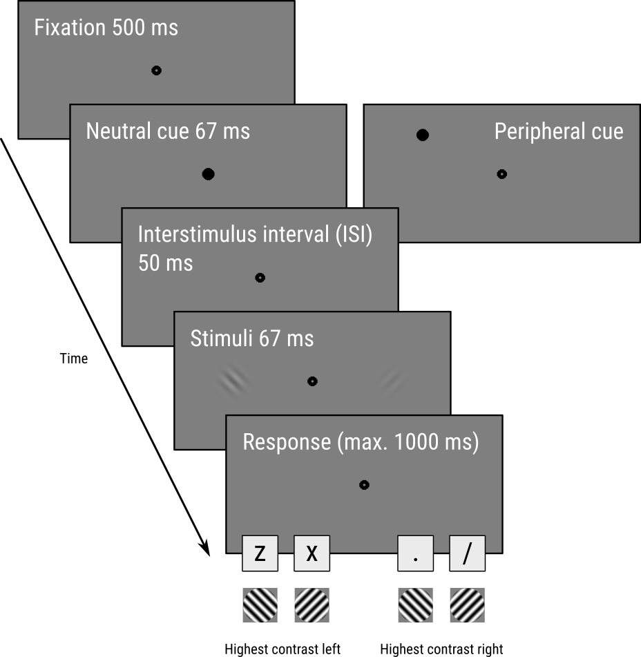
Figure 1. The trial sequence, based on Carrasco, Ling, and Read (2004) with slight adapations.

Building the experiment

Step 1: Add a block_loop and trial_sequence

When starting OpenSesame, the default template is automatically opened. The default template starts with three items: A notepad called getting_started, a sketchpad called welcome, and a sequence called experiment. We don't need getting_started and welcome, so let's remove these right away. To do so, right-click on these items and select 'Delete'. Don't remove experiment, because it is the entry for the experiment (i.e. the first item that is called when the experiment is started).

Our experiment will have a very simple structure. At the top of the hierarchy is a loop, which we will call block_loop. The block_loop is the place where we will define our independent variables. To add a loop to your experiment, drag the loop icon from the item toolbar onto the experiment item in the overview area.

A loop item needs another item to run; usually, and in this case as well, this is a sequence. Drag the sequence item from the item toolbar onto the new_loop item in the overview area. OpenSesame will ask whether you want to insert the sequence into or after the loop. Select 'Insert into new_loop'.

By default, items have names such as new_sequence, new_loop, new_sequence_2, etc. These names are not very informative, and it is good practice to rename them. Item names must consist of alphanumeric characters and/ or underscores. To rename an item, double-click on the item in the overview area. Rename new_sequence to trial_sequence to indicate that it will correspond to a single trial. Rename new_loop to block_loop to indicate that will correspond to a block of trials.

Finally, click on 'New experiment' to open the Experiment Properties. Click on the title of the experiment, and give it an informative name, such as 'Attention alters appearance'.

The overview area of our experiment now looks as in Figure 2.

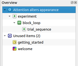
Figure 2. The overview area at the end of Step 1.

Step 2: Defining experimental variables in the block loop

Our experiment has five experiment variables (or: independent variables, factors, conditions):

• test_contrast determines the contrast of the test stimulus, which in the original experiment was varied between 6% and 79% in 23 logarithmically spaced steps (i.e. as the contrast gets higher, the distance between subsequent contrast levels also increases). 23 levels is a bit much, so here we will stick to a more manageable 6 steps, which are also logarithmically spaced. Expressed in proportions as opposed to percentages, this gives the following values: .06, .10, .17, .28, .47, and .79
• cue determines whether the task-irrelevant cue appears above the location of the standard stimulus, the test stimulus, or the fixation dot. This gives the following values: standard, test, and neutral
• standard_ori indicates the orientation of the standard stimulus in degrees of clockwise rotation relative to the vertical. This gives the following values: -45 and 45
• test_ori is the same but then for the test stimulus.

We also need to define which stimulus appears where: the standard on the left and the test on the right, or vice versa. There are many different ways to do that, but an easy solution is to define the x-coordinate of the standard patch. (The x-coordinate of the test patch then doesn't need to be defined, because it's always on the opposite side.)

• standard_x gives the x-coordinate of the standard patch in pixels relative to the center of the screen. We can use the following values: -128 and 128

Together, these experimental variables make up a fully crossed (or: full-factorial) 6 (test_contrast) × 3 (cue) × 2 (standard_ori) × 2 (test_ori) x 2 (standard_x) design, which means that we have 144 distinct combinations.

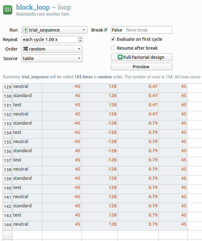
Figure 3. The loop table.

Step 3: Adding items to the trial sequence

Right now, trial_sequence is empty, that is, it doesn't contain any items that actually implement a trial. So let's do that now.

We need five static displays as shown in Figure 1:

• Fixation display with just a fixation dot
• Cue display with a fixation dot and the cue
• Inter-stimulus-interval (ISI) display again with just a fixation dot
• Stimulus display with a fixation dot and the two stimuli
• Response display again with just a fixation dot

Static displays correspond to sketchpad items. Therefore, drag five sketchpad items from the item toolbar onto trial_sequence. Give them sensible names, such as fixation_sketchpad, cue_sketchpad, etc. Don't do anything else with these sketchpad items for now.

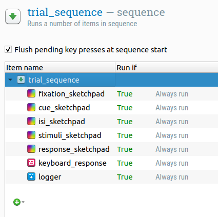
Figure 4. The overview area after adding all items to the trial_sequence.

Step 4: Adding fixation dots and durations to the sketchpad items

This step is purely DIY!

Step 5: Defining the cue

Now that each sketchpad has a central fixation dot and an appropriate duration, we still need to define the cue and the stimuli.

Open the cue sketchpad. The cue should be a small, black filled circle that either appears just above the location where one of the stimuli will appear, or at the location of the central fixation dot.

First, draw a small filled black circle at the location of the fixation dot. This will be our neutral cue. Right now, the show-if expression for this stimulus is True, which means that it is always shown. However, we want the stimulus to be shown only when the variable cue has the value 'neutral'. To indicate this, change the show-if expression to:

cue == 'neutral'

This show-if expression is a Python expression that checks whether the variable cue has the value 'neutral'.

Next, draw another cue just above the midline on the left side, at location -128, -64. This will serve as both the standard and test cue, so change the show-if expression for the stimulus so that it is shown only when the cue is not neutral:

cue != 'neutral'

Now it's time to look at a special feature of OpenSesame: the ability to view and edit the script that defines an item. You can do so by clicking on the drop-down button at the top-right (next to the help button) and selecting 'Split view'. This will open a script editor at the bottom of the window. Importantly, this script is not Python script, but OpenSesame script: a simple domain-specific language that is used to the define experiments. The script and the user interface are linked: if you change something in the script, the interface will change along, and vice versa.

We'll use the script to have the x-coordinate of the cue depend on the standard_x variable. Specifically, the x-coordinate should be equal to standard_x if the variable cue has the value 'standard', and be equal to -standard_x (i.e. on the opposite side of the screen) otherwise. This corresponds to the following Python expression:

standard_x if cue == 'standard' else -standard_x

To embed this Python expression in the OpenSesame script, we need to put it between {curly braces}. This is a so-called F-string (or: template literal): a string of text where everything between curly braces is interpreted as a Python expression.

draw circle color=black fill=1 penwidth=1 r=10 show_if="cue != 'neutral'" x="{standard_x if cue == 'standard' else -standard_x}" y=-64.0 z_index=0

Note that the show-if expression is not put between curly braces. This is because a show-if expression is always a Python expression, whereas an x-coordinate is not: rather, it is a value that may or may not include a Python expression.

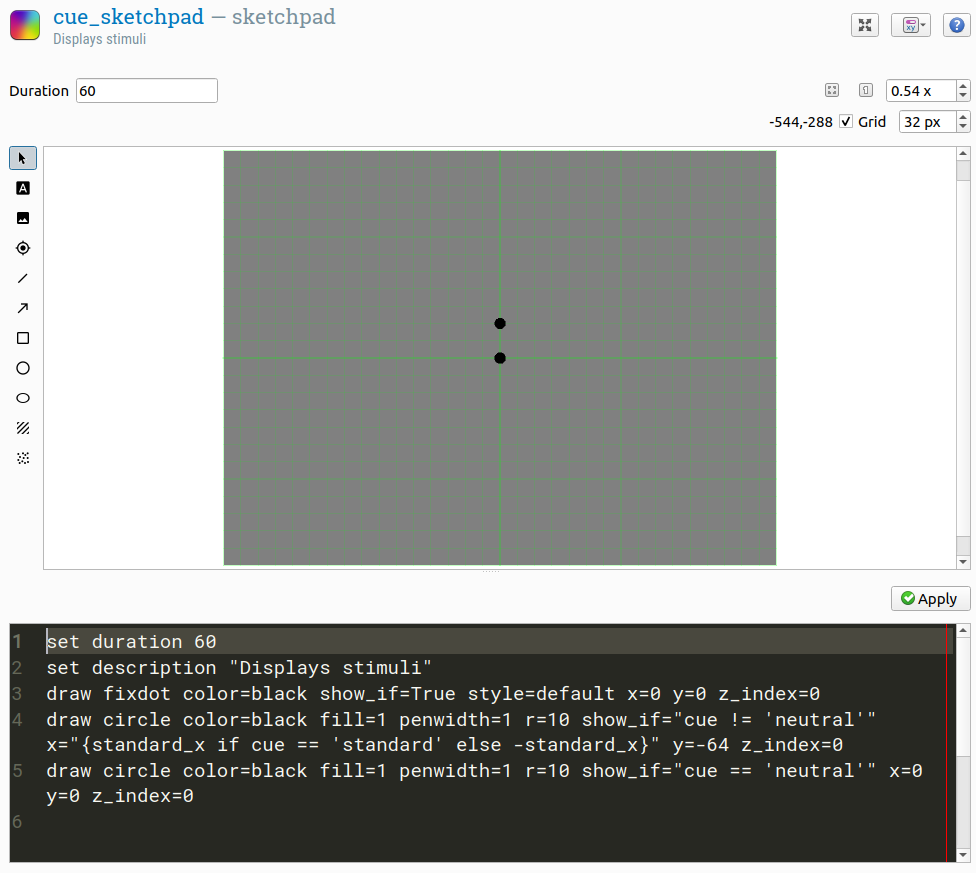
Figure 5. Split view of the cue_sketchpad item.

Step 6: Defining the standard and test stimuli

Open the stimuli sketchpad. Draw two gabor patches, one at location -128, 0 and one at location 128, 0. In the configuration dialogs that appear, you can leave the settings on their default values. Next, as before, open the split-view so that you can see both the user interface and the item script.

The first gabor patch will serve as the standard stimulus. This means that we need to use the variables standard_ori and standard_x for respectively the orient and x parameters. We also need to specify two color parameters: color1 and color2. To understand what these parameters mean, it's useful to think of a gabor patch as a texture that oscillates between two colors; if one of these colors is white and the other is black, then you get the typical high-contrast gabor patch; if one of these colors is dark gray and the other is light gray, then you get a gabor patch with less contrast; you can also create more exotic gabor patches that oscillate between different colors, such as red and blue.

In OpenSesame, you can define colors in many different ways, one of which is as a number between 0 (black) and 255 (white), where 128 is an intermediate gray. In our case, the standard stimulus has a contrast of 22%. What does this mean in terms of color values? It means an oscillation from 128 - .22 × 128 ≈ 100 to 128 - .22 × 128 ≈ 156.

Taken together, we need to adjust the script for the standard stimulus as follows:

draw gabor bgmode=avg color1=100 color2=156 env=gaussian freq=0.06 orient="{standard_ori}" phase=0 show_if=True size=96 stdev=12 x="{standard_x}" y=0 z_index=0

Step 7: Configuring the keyboard_response

This step is purely DIY!

Testing the experiment

Doing a test run

There are two main ways to run the experiment:

• The blue quick-run button launches the experiment in a window without asking for a participant number or log file. You typically use this to test your experiment during development.
• The green run button first asks for a participant number and log file and then launches the experiment fullscreen. You typically use this to collect data in the lab.

Click on the quick-run button. If you've followed the tutorial accurately, the experiment should now launch in a window. (And if it doesn't, don't worry: we'll deal with error messages shortly.)

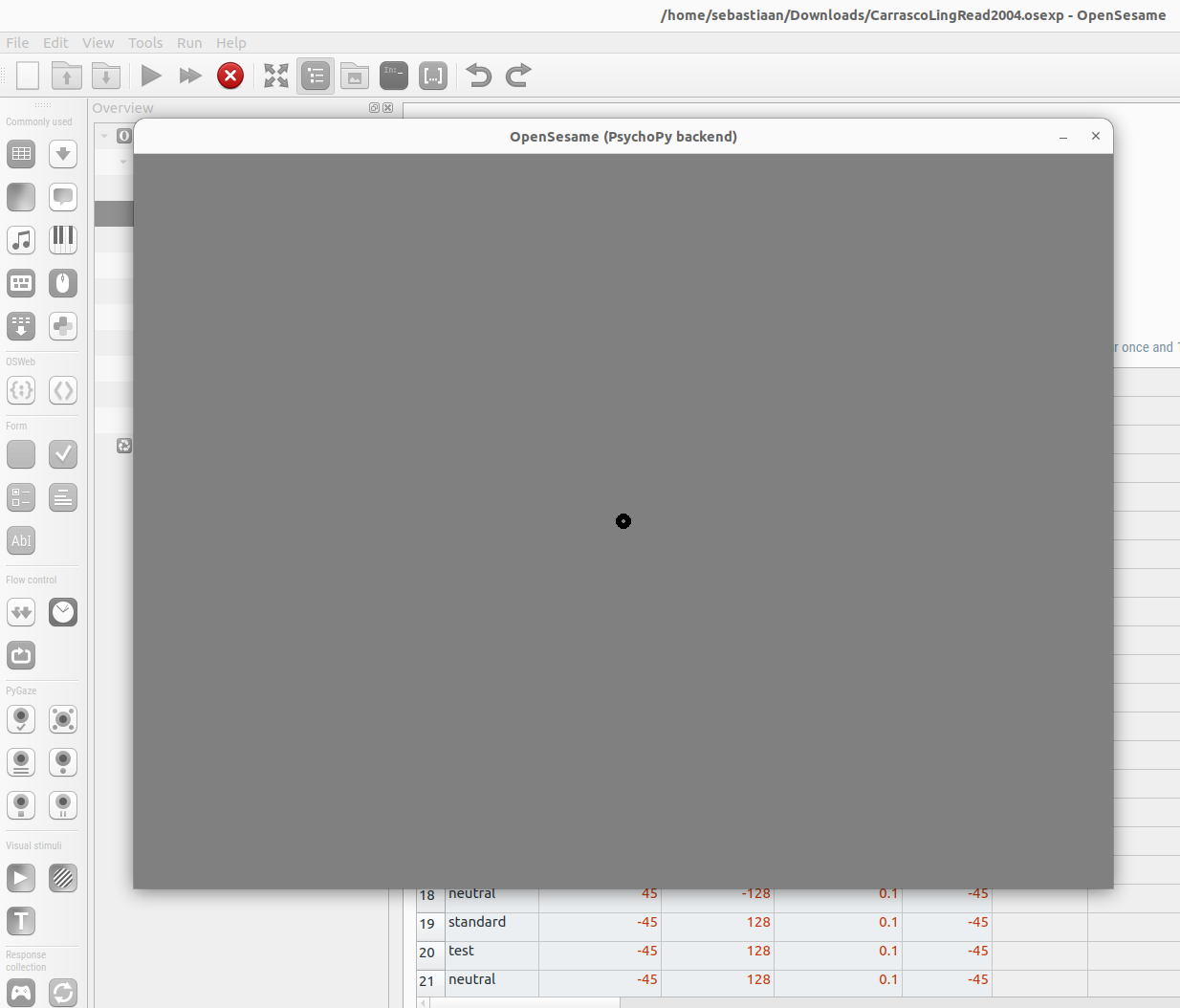
Figure 6. The quick-run button launches the experiment in a window for testing.

To abort the experiment, either press q (and then y to confirm) or click the red kill button to immediately close the experiment.

Understanding error messages

Understanding and fixing errors is a crucial skill when developing your experiment. Let's intentionally introduce a bug in order to see and understand error messages in OpenSesame: open the block_loop and rename the variable cue to queue; this simple typo is characteristic of the kind of bugs that you will frequently encounter. If you now run the experiment again, it will crash with the following error:

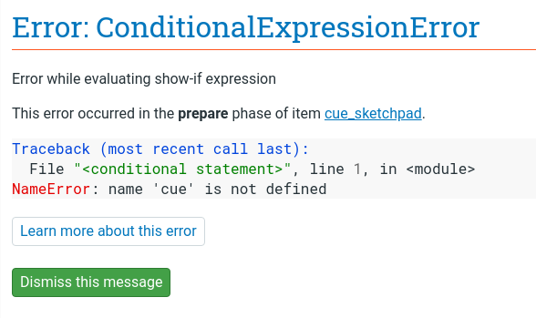
Figure 7. A ConditionalExpressionError indicates an issue when trying to evaluate a conditional expression, such as a show-if expression.

This is a ConditionalExpressionError, which means that there was a problem while evaluating a conditional expression, which includes run-if, show-if, and break-if expressions. The error further clarifies that the error results from a show-if expression in cue_sketchpad, and, more specifically, that cue is not defined.

With this in mind, and after inspecting show-if statements in the cue_sketchpad item, it should become clear what is wrong (even if we hadn't intentionally introduced the error): the show-if statement refers to a variable called cue, whereas the block_loop defines a variable called queue. You can then proceed to fix this by changing the name of the variable in cue_sketchpad or (more sensibly) in block_loop.

Verifying timing through timestamps

Temporal precision of stimulus presentation is important in many experiments. That is, you often need to be able to control and verify exactly when stimuli appear on the screen. OpenSesame provides excellent temporal precision in general; however, temporal precision depends on both software and hardware, and therefore it is important to check timing on your own experimental setup.

To see how you can do this, let's start by collecting a log file from a short test run. Perform this test run in full screen, which can make a difference in terms of timing.

Once you have completed a test run, open the resulting log file. In this example, the log file is called subject-0.csv and contains 14 trials. We'll open the file with Python DataMatrix, but you can also use Excel, R, DataFrame, JASP, or some other library that is able to read .csv files:

from datamatrix import io
dm = io.readtxt('subject-0.csv')

Most items in OpenSesame automatically create a variable called time_{item_name} that keeps track of 'when the item happened'. In the case of sketchpad items, this corresponds to the onset timestamp of the display. Let's print out time_fixation_sketchpad, which contains the onset timestamps for fixation_sketchpad.

# Print out the onset times of cue_sketchpad
print(dm.time_fixation_sketchpad)

Out:

col[3913.7363729969366, 5323.123084999679, 6759.262975996535, 8488.704181996582, 9874.551597997197, 11039.999496999371, 12273.833031998947, 14011.335637995217, 15741.652134995093, 17161.13185499853, 18337.58171500085, 19489.91102299624, 20775.85124199686, 21971.585808998498]

These timestamps are not by themselves very informative. However, by subtracting them from the onset timestamp of the next sketchpad, we get the presentation duration. In other words, the onset timestamp for cue_sketchpad minus the onset timestamp for fixation_sketchpad is equal to the presentation duration of fixation_sketchpad. Let's take a look:

# Print out the presentation durations of fixation_sketchpad
fixation_duration = dm.time_cue_sketchpad - dm.time_fixation_sketchpad
print(fixation_duration)

Out:

col[500.0524060014868, 499.5914620012627, 500.36454899964156, 499.8691369983135, 500.2033729979303, 500.30748100107303, 500.34059100289596, 500.16464500367874, 499.92641800054116, 500.20127100287937, 500.24507999478374, 500.29579600231955, 500.31029700039653, 500.4937609992339]

A few things stand out here. First, presentation durations are very constant, not once deviating more than 0.5 ms from 500 ms. Second, presentation durations are not 495 ms, which we had indicated as the duration of fixation_sketchpad, but rather 500 ms. Does this indicate a problem with timing?!

In fact, a presentation duration of 500 ms is exactly what we would expect given the 60 Hz refresh rate of the monitor. A display can only be presented once every refresh cycle. On a 60 Hz monitor this means that presentation durations are necessarily multiples of 16.6 ms (= 1000 ms / 60 Hz): 16.6 ms, 33.3 ms, … 483.3 ms, 500 ms, etc. In other words, a duration of 495 ms is not possible, and will therefore be rounded up to the nearest possible presentation duration, which is 500 ms.

You can read more about the intricacies of timing here. But for now the golden rule to keep in mind when specifying sketchpad durations is: specify a duration that is slightly (say 5 ms) less than the intended duration!

Let's determine the presentation durations for the other sketchpad items and visualize them in a figure:

import numpy as np
from matplotlib import pyplot as plt

# Determine the presentation durations of the remaining sketchpads
cue_duration = dm.time_isi_sketchpad - dm.time_cue_sketchpad
isi_duration = dm.time_stimuli_sketchpad - dm.time_isi_sketchpad
stimuli_duration = dm.time_response_sketchpad - dm.time_stimuli_sketchpad

# Plot them and draw horizontal lines to indicate the intended presentation
# duration
plt.plot(fixation_duration, color='blue')
plt.axhline(500, linestyle=':', color='blue')
plt.plot(cue_duration, color='green')
plt.axhline(67, linestyle=':', color='green')
plt.plot(isi_duration, color='red')
plt.plot(stimuli_duration, color='purple')
plt.axhline(50, linestyle=':', color='gray')
# Draw ticks on the Y axis every other frame
frame_duration = 1000 / 60
plt.yticks(np.arange(0, 550, 2 * frame_duration))
plt.ylabel('Presentation duration (ms)')
plt.xlabel('Trial nr')
plt.show()

Out:

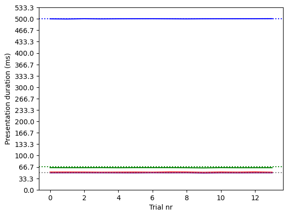
Figure 8. Actual and intended presentation durations in our short test run.

The figure above shows that for each sketchpad and on each trial, the actual presentation duration (solid lines) was almost exactly the intended presentation duration (dotted lines). Since a real temporal deviation has to be at least one frame duration (16.6 ms), this means that very small, submillisecond deviations are due to other factors and do not reflect any true temporal imprecision. In other words, in this short test run and as far as we can tell based on timestamps, temporal precision was literally perfect!

Verifying timing through external measurement

When verifying timing through timestamps, as we have done above, we are relying on the computer's ability to know when things appear on the display. But the computer cannot always know this. For example, the monitor itself may contain software that affects timing, and this would not be reflected in the timestamps. Therefore, in order to comprehensively check display-presentation timing, you need to use an external device, such as a photodiode, that registers when things actually appear on the display.

Finished

This concludes the workshop! I hope you found it useful and have fun at the conference!

Additional exercises

Giving feedback

Right now, participants do not receive feedback on their responses. They apparently didn't in the original study by Carrasco and collagues either; however, providing feedback is a good to increase the motivation of participants. Therefore:

• Define a correct_response variable to indicate which key participants are supposed to press. You can define this variable directly in block_loop, or you can use a short (Python) inline_script to determine the correct response based on the variables standard_x, test_contrast, standard_ori, and test_ori.
• At the end of each trial, briefly show a green fixation dot when the response was correct, and a red fixation dot when the response was incorrect.

Having shorter blocks

Right now, block_loop consists of 144 trials that are executed without interruption. Your participants deserve a break every once in a while! Therefore, subdivide the experiment into multiple, shorter blocks.

Do not set the repeat value for block_loop to less than 1. This will shorten the blocks, but it will do so by randomly sampling from possible trials, and thus not guarantee that all possible trials occur equally often. Instead:

• Either use a break-if expression in combination with the resume-after-break option in block_loop.
• Or add a break sketchpad to the trial_sequence and use a run-if expression to make sure that it appears only after a fixed number of trials.

Running your experiment online

This experiment can be executed in a browser almost straight away!

• If you have used an inline_script, you first need to translate this to an inline_javascript.
• Test the experiment in a browser on your own computer
• Finally, publish the experiment to a JATOS server, such as MindProbe.eu, create a link that you can share with participants.

References

Carrasco, M., Ling, S., & Read, S. (2004). Attention alters appearance. Nature Neuroscience, 7(3), 308–313. https://doi.org/10.1038/nn1194
Mathôt, S., Schreij, D., & Theeuwes, J. (2012). OpenSesame: An open-source, graphical experiment builder for the social sciences. Behavior Research Methods, 44(2), 314-324. https://doi.org/10.3758/s13428-011-0168-7